This tutorial was originally posted to the Roblox DevForum’s, and this version is adapted to the website.

Hello everyone!

Major disclaimer before we begin: This tutorial is meant to teach people the basics of ML and how it can be applied to Roblox, this is NOT a proper anti-cheat for your games!

*Oh, also, please note that in this scenario, you’d be better off not using ML in this example, but there are plenty of situations where you definitely could & should

What you’ll need:

Python 3
An ML library of your choice (or none if you like linear algebra and calculus)
Basic knowledge of Lua

We’ll be using TensorFlow & Keras in this tutorial, but honestly because we’re making an MLP, this is easy to follow along in any framework! Anyways, with that out of the way, let’s get to…

Our Problem

Let’s say we have this cool obby game that people like to speedrun. To empower moderators, we create a system that records the players position on the server at every second, and save this data. Typically, moderators are able to hand pick exploiters from the in-game leaderboards. Suddenly, a huge swath of exploiters come and run rampant! If only there was a way to flag runs for moderators to quickly identify exploiters…

picture of the obby game

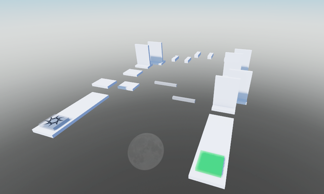
We could use invis-checkpoints, but that’s lame (and more practical), so let’s use ML to solve this! We’re going to make a model that can look at a series of positions from a player, and determine if they are likely exploiting. But first, we need to understand and collect…

Data

Alright, so this is our very first step. In order to build a good ML model, we’ll need data, and more specifically 'cause we’re going the supervised route, we’ll need labeled data. What this means is we need to not only record player position data, but also include whether or not they were “exploiting”. In this case, exploiting just means using a NoClip tool, and we’ll just note down if we did or didn’t use it.

I don’t have a game with hundreds of players and an attentive mod team, so let’s synthesize some! This is the script I used to generate mock-data:

local Players = game:GetService("Players")
local HttpService = game:GetService("HttpService")

local winpad = workspace:WaitForChild("Winpad")

local data = {}
local active = true

-- yes ik this isn't a good way to do this, but for my purposes,
-- this will do fine! if you were to legit do this, see if you can
-- account for lag, and obviously only record player data when needed :)
function roundVector3(vector)
	local roundedX = tonumber(string.format("%.2f", vector.x))
	local roundedY = tonumber(string.format("%.2f", vector.y))
	local roundedZ = tonumber(string.format("%.2f", vector.z))
	
	return `{roundedX},{roundedY},{roundedZ}`
end

Players.PlayerAdded:Connect(function(player)
	player.CharacterAdded:Connect(function(character)
		local humanoidRootPart = character:WaitForChild("HumanoidRootPart")
		
		winpad.Touched:Connect(function(obj)
			if obj.Parent == character and active then
				active = false
				local roundedPosition = roundVector3(humanoidRootPart.Position)
				table.insert(data, roundedPosition)

				local output = table.concat(data, "%")
				
				-- point of this is to be able to easily store our data as a string
				print(output)
			end
		end)
		
		while active do
			task.wait(1)
			
			local roundedPosition = roundVector3(humanoidRootPart.Position)
			table.insert(data, roundedPosition)
		end
	end)
end)

Ok cool! With that script, I just saved the output of some regular runs, and some “exploiter” runs. I split evenly, and did 10 normal and 10 exploiting.

top down paths

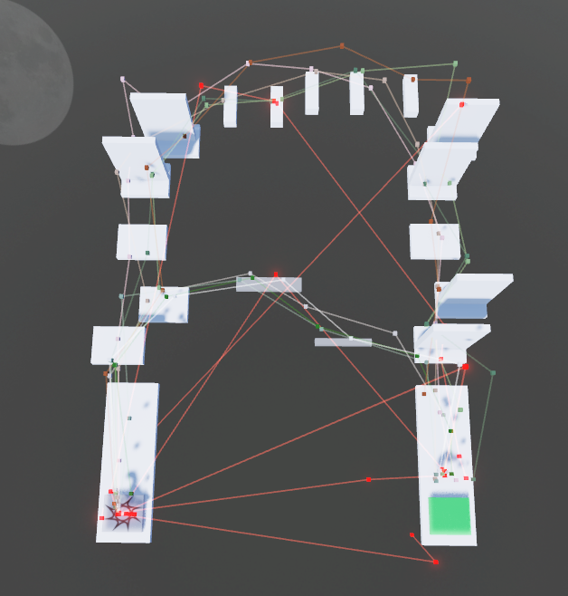
All paths that are red & neon are exploiter paths, and paths that are other colors are normal. Notice how the red ones typically cut through large portions of the obby, whereas normal paths either follow the top or bottom path. Pretty cool, right? These are the patterns we’re hoping for the model to pick up on.

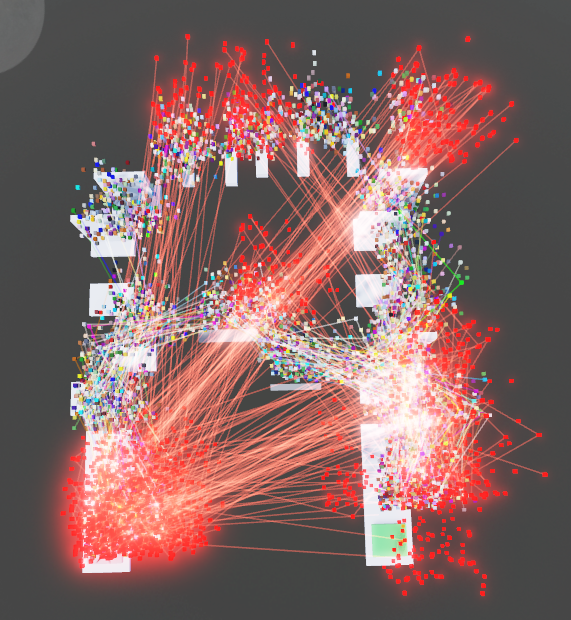
But here’s the thing, 20 runs isn’t going to cut it! We’ll need a ton more, and because I can’t spend my entire day playing this obby, we can instead add random noise to our data to make more of it. Essentially, at each point, we offset it by a random amount in the X, Y, and Z axes. I generated 70 per normal path giving us a total of ~1.2k runs.

Noise data (player generated is much better, but this will do for now!):

trends

Alright cool!

Important Decision

Do you want to train the model within or outside of Roblox?

If you train the model within, you may need to restructure your data a little differently, but from there on out you can use DataPredict by @MYOriginsWorkshop, or really any other ML library on Roblox.

For the rest of this tutorial, I’m doing this outside of Roblox, but don’t worry if you aren’t. You can skip the data exporting, and can roughly follow along with the ML steps.

Data Exporting

Let’s export this to a CSV. To do so, we’re going to use GitHub gists. In order to create the export code, we can read this cool guide by @astralboy.

If you don’t know, Gists are a cool thing made by GitHub that allow you to have a file that can be read/written to externally! While their use-case typically isn’t that, they have provided an end-point so it’s fair game for something like our purpose :). If you don’t have a GitHub account, I highly recommend you get one. They’re free, and can also get you into the awesome world of Git and version control. Anyways, here’s our code for exporting the data:

⚠️ LAG WARNING: Pushing this much data causes some pretty hefty lag for a couple seconds, I recommend exporting your data a different way if you don’t have a great internet connection/computer! ⚠️

finalPaths = -- whatever your final paths are!

local AUTH = "AUTH_TOKEN_HERE"
local URL = "GITHUB_GIST_URL_HERE"

local headers = {
	["Authorization"] = `Bearer {AUTH}`
}

local patch = HttpService:RequestAsync({
	Method = "PATCH",
	Url = URL,
	Headers = headers,
	Body = HttpService:JSONEncode({
		files = {
			["main.csv"] = {
				-- filename is whatever you named your gist file
				content = finalPaths
			}
		}
	})
})

-- seeing what happened to it
print(patch)

Alright, after a few seconds of lag, you should’ve gotten a 200 (OK), which means our data has exported successfully.

Data Processing

To make our data easier to handle, we’re going to need to whip up a data parser that takes in our “raw” data and converts it to a proper CSV format. Why CSV? Well, it’s pretty much the universal file format for data like this, as it has a large ecosystem of tools within python to interact with it, and load it into our model much faster. Essentially, what happens is…

roblox format (raw)	csv format (what we want)
false,1,2,3%3,6,2%…	time,is_exploiting,x,y,z
	1, 0, 1, 2, 3
	1, 0, 3, 6, 2
	etc…

We’re going to be using pandas which is a python library that allows us to handle CSVs much easier to help us with this.

# data-parser.py
import pandas as pd 
import re
import csv

data = pd.read_csv("PATH_TO_YOUR_DATA", header=None, sep=" ", quoting=csv.QUOTE_NONE, on_bad_lines="skip")

to_replace = {
    "false": "\nfalse",
    "true": "\ntrue",
    "%": "\n",
}

for value, replace in to_replace.items():
    drop = True if value == "%" else False

    data[0] = data[0].str.replace(value, replace).str.split("\n")
    data = data.explode(0).reset_index(drop=drop)

previous_is_exploiting = "false"
current_time = 0

# just doing it this way to force the order
data.insert(0, "time", "")
data.insert(1, "is_exploiting", "")
data.insert(3, "x", "")
data.insert(4, "y", "")
data.insert(5, "z", "")

for index, row in data.iterrows():
    modifier = 0

    # because of our data structure, each row should have whether or not it's an exploiters
    # run, so that's what we're doing here
    if "false" in row[0] or "true" in row[0]:
        is_exploiting = 0 if "false" in row[0] else 1

        modifier += 1
        current_time += 1
        
        previous_is_exploiting = is_exploiting
        data.at[index, 0] = data.at[index, 0].replace(f"{is_exploiting},", "")

    data.at[index, "time"] = current_time
    data.at[index, "is_exploiting"] = previous_is_exploiting

    split = row[0].split(",")

    if len(split) >= 3 + modifier:
	    # force rounding it, you could honestly drop this part, because lerp 
	    # will remove the rounding anyways
	    
        data.at[index, "x"] = "{:.2f}".format(float(split[0 + modifier]))
        data.at[index, "y"] = "{:.2f}".format(float(split[1 + modifier]))
        data.at[index, "z"] = "{:.2f}".format(float(split[2 + modifier]))

data = data.drop(columns=["index", "level_0", 0])
data.to_csv("PATH_TO_EXPORT.csv", index=False)

Right now, we have another huge issue: for the model architecture we are using, we want our data to be the same chunk size! What do I mean? Essentially, because some players are able to complete the obby in say 4 seconds, where others complete it in 7 and so on, we want some way to make sure all runs have the “same” time length. We also don’t want the model to learn “less time = hacking”, and I’m sure you can see why. I’ll be choosing 15 (because it’s my longest data-point), but this really depends on your use case, and which runs you consider to pick for monitoring. So to make all of our runs the same length, we can do some interpolation.

Mini lesson on linear-interpolation

What is it? Essentially, linear interpolation or “Lerp” is where we try to estimate a point between two known points. I could give you the mathematical definition and all of that, but I feel it’s pretty intuitive from that alone. So how can we use this? Well, because we want all runs to have 10 data-points, we simply look at the ones that don’t, and Lerp the in-between. Obviously, you can imagine that this gets more and more inaccurate, so we need to be careful in how we choose our “magic number” that we align our data too. Too high, and lots of our data’s intricacies will be lost!

Here we’ll be using numpy to handle our linear interpolation.

# data-lerp.py
import pandas as pd
import numpy as np

target = 15

def lerp_chunk(chunk_df):
    # if it's already 15, ignore!
    if len(chunk_df) == target :
        return chunk_df

    linspace = pd.DataFrame(
        index=pd.RangeIndex(target),
        columns=chunk_df.columns
    )

    linspace["time"] = chunk_df["time"].iloc[0]
    linspace["is_exploiting"] = chunk_df["is_exploiting"].iloc[0]

    for col in ["x", "y", "z"]:
        linspace[col] = pd.Series(np.interp(
            np.linspace(0, 1, num=target_rows),
            np.linspace(0, 1, num=len(chunk_df)),
            chunk_df[col]
        ))

    return linspace

df = pd.read_csv("PATH_TO_ORIGINAL_DATA.csv")
df.sort_values(by=["time"], inplace=True)
result_df = df.groupby("time", group_keys=False).apply(lerp_chunk)

result_df.reset_index(drop=True, inplace=True)
result_df.to_csv("PATH_TO_LERPED_DATA.csv", index=False)

Alright so after running that, we should now have our newly lerped data. If you open up the CSV, you should notice all the chunks/runs are exactly 15 points, and that the points from our original data are kept.

Here’s a quick graph I made using matplotlib (only plotting X & Z, technically they’re flipped but oh well, you get the point):

lerped vs unlerped data

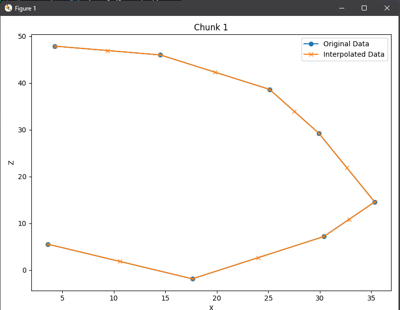
Notice how it kept our original data, and only added new data where it’s needed to add up exactly to 15? That means it works! If this example looks great, what did I mean “too much interpolation can cause us to lose intricacies in our data”? This comes down to plotting this against our actual obby. Due to us only recording every 1 second, things like wraparounds are completely ignored, so it looks like we just walked right through them. With the original data, all the points are valid positions the character may be at, but with the interpolated data, they may have invalid positions.

This is why if minute details like this really do matter, you might want to consider other model types such as LSTMs that don’t require “even” data.

For our purposes, this model should learn fine regardless of these “invalid” positions. Ok well, here’s the moment this entire tutorial has been leading to. Are you ready? Because now it’s time for…

Machine learning

Woah, I said the scary word! Don’t worry, we’ll be using one of the simplest model architectures, and I’ll explain the math as we go.

If you really couldn’t care less about what’s actually going on, skip to “Creating the model”. But, I highly recommend everybody who doesn’t understand the math behind our model to read this next part thoroughly!

What’s actually happening?

Let’s say we have a new, simpler scenario. We have X (amount of time a player has spent in game), and we want to predict Y (the amount of currency they have). Well, assuming that our currency progression is pretty linear, we might use the classic

$y=mx+b$

Where we can imagine “y” and “x” to be our currency and player time respectively. From this, we can create the basic setup of…

time spent, mx * b, amount of currency

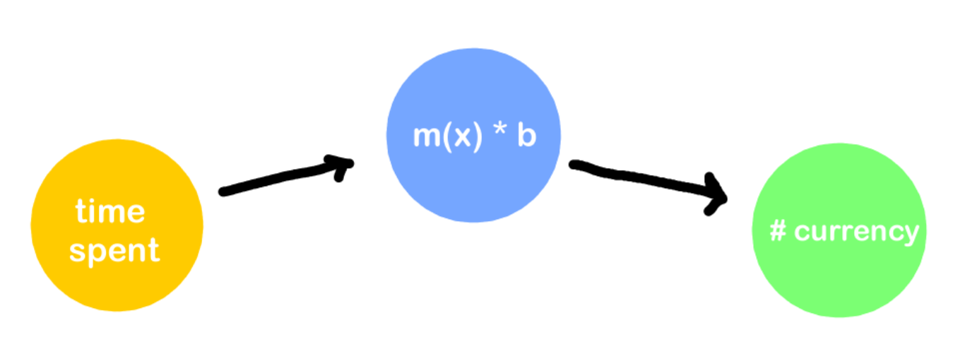
One issue though, how do we find our magic “m” and “b” to make this true? It’s relatively easy to brute force for 1 specific value, but let’s say we have 100 on a scatter plot, how can we do it? What we need to do is make our system “learn”. The very first step to learning is to see where and how we went wrong, so in our case, we should figure out how “wrong” our model was (essentially giving it a grade).

We have to start somewhere, so we’ll just randomize the values of m & b. Yes, this does inherently mean that sometimes when you train a model, it will do better than a previous time because it got more lucky, but typically the actual performance gained will be minuscule.

Back to our grading system; a pretty simple way to start is to take the difference between what we predicted (O) and observed ( P ). “i” here just means the index.

$O_{i}-P_{i}$

Next, because we want a single score and not a score for each point, let’s do this for each data-point & take the sum of it all.

$um^{n}{i=1} O{i} - P_{i}$

If you’re confused, the weird sideways looking M is sigma notation, which is a fancy way that allows us to condense huge summations.

Alright, and with that we have a loss function, but it’s not really the best. The reason is why is because the negatives and positives could cancel each other out. A much better, and more classic way to calculate this “score” is through the mean squared error (MSE) function.

$athrm{MSE} = rac{1}{n} um_{i=1}^{n}(Y_{i}-at{Y}_{i})^2$

This looks a lot scarier than our simple function, but the additional changes are really basic!

The Y with the little hat on it is the same as our P, and the normal Y is our O
The reason we’re squaring each one is to essentially amplify the model’s shortcomings, and force it to work well with the entire dataset.
It gets multiplied by 1 over the number of data-points, and this is just to make the dataset’s size irrelevant to loss. Look at our original function, if we had a model with the same accuracy, but one dataset with 100 points and one with 10 points, it would naturally get a much better loss score on the lower dataset. Dividing by n allows us to avoid this.

Now that we have a fancy way of telling how bad our model is, how do we actually use this to tell the model to get better?

Gradient descent & back propagation

Due to how long this tutorial is getting, we will not be taking a deep dive into back-propagation, but instead I’ll link some really helpful resources!

Tying this back into our model

Deep Learning

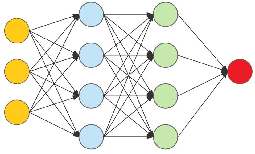
Ever seen this classic diagram when discussing machine learning? It’s often the quintessential representation of a Multi-layer Perceptron (MLP), but it looks a lot scarier than what we just made! But what if I told you the model we made is really close to this, all we need to do is add more of those middle layers.

What if we had 1 input (the yellow circles) for each X, Y, or Z component in our data (so 15 * 3 inputs)? Then, we could have however many inside neurons (commonly called “the hidden layers”), and have each of our inputs connect to one neuron.

Remember, all a hidden neuron does is apply an equation to its inputs. In this case, because it has multiple inputs, we’d do “(m1 * x) + (m2 * x) + (m3 * x) … (m15 * x)” and then finally add “b” to the sum of all of that. Notice how we already have a lot of power just from our first hidden layer, and don’t really need the second one (the green one). This is one of the really cool things about machine learning, you get to play and design with how your model works! For your case, you might need 2, or maybe even 3 hidden layers, but for ours, this model is strong enough to just have 1.

Last critical thing: Right now, what we’re doing is a regression, because we have no non-linearity in our network. What does this mean? Well, if our entire networks are based on lines, what if our data isn’t just linear, and has more underlying patterns? To quickly add a non-linear aspect, we use something called an activation function. Activation functions get run just after “exiting” our hidden neurons.

But what is f(x)? In theory, whatever you want!

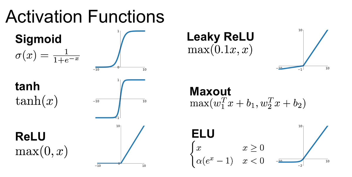
Introduction to Different Activation Functions for Deep Learning | by Shruti Jadon | Medium

Here are some common ones you’ll most likely see in the field. Notice how all of them attempt to do something to break the linear pattern, like Sigmoids skewing data to be either 0 or 1, or ReLU eliminating negative numbers.

Finally, as for our output neuron (the red circle), we’ll just have 1. This is because we’re trying to predict whether or not the run given in the outputs was an exploited run (which can easily be represented as 0 or 1). The closer our last neuron is to 1, the more likely they are cheating, and vice versa.

Creating the model!

You can skip this if you aren’t using TensorFlow or are doing this on Roblox :^)

TensorFlow is a tool that allows us to construct the models we made above into actual working ones through python. After following the instructions from [https://www.tensorflow.org/install/pip], you’re good to start making the model!

What we’ll be doing is using Keras (which comes with TensorFlow) to build it. While it’s always nice to build from scratch, this tutorial is getting really long, and this provides a nice abstraction! Think of it like being able to declare our model architecture with English, rather than math.

import  pandas  as  pd
import  numpy  as  np
import  tensorflow  as  tf

from  tensorflow  import  keras
from  keras.layers  import  Dense

data  =  pd.read_csv("data/lerped-data.csv")

# Making sure the chunks are 15 long!
positions  =  data[["x", "y", "z"]].values.reshape(-1, 15, 3)
is_exploiting  =  data["is_exploiting"].values[::15]

# Splitting the data into a training set, and a test set to see how well we did!
split  =  int(len(positions) *  0.8)
shuffle_index  =  np.random.permutation(len(positions))

positions, is_exploiting  =  positions[shuffle_index], is_exploiting[shuffle_index]

positions_train, positions_test  =  positions[:split], positions[split:]
is_exploiting_train, is_exploiting_test  =  is_exploiting[:split], is_exploiting[split:]

And with that out of the way, here’s our model!

model  =  keras.Sequential([
	keras.layers.Flatten(input_shape=(15, 3)),
	keras.layers.Dense(64),
	keras.layers.Dense(1, activation="sigmoid")
])

model.compile(optimizer="adam",
	loss="binary_crossentropy",
	metrics=["accuracy"])

model.fit(positions_train, is_exploiting_train, epochs=15, batch_size=15)

Wait what? That’s it? What just happened? Well even though the code looks a bit confusing, I’ve already taught you everything in this! The keras.Sequential() sets up a model that’s layer-after-layer. Our Flatten layer takes our 15x3 “rectangle” and squishes it to be 45 with no 2nd dimension. This makes it easy to feed into our Dense layer, which is 64 of those little circles we thought of above! Finally, all of it comes to 1 node on a dense layer. If it’s closer to 0, their not hacking, if 1, then they are!

The compilation allows us to ask for the metrics we want from the model (accuracy), how it’s evaluated (binary_crossentropy), and the algorithm doing it (adam). I discussed gradient descent which is the basic principle, but adam is a more elaborate version.

When we “fit” the model, we’re just constantly forward propagating and back propagating along our dataset to train it. We then do this process for epoch=15 times and voila. Just like that, we’ve collected, cleaned, analyzed data and trained a binary choice multi-layer perceptron to determine whether someone exploited in an obby. I know, these are all big fancy words, but it’s true!

After our final evaluation, we figure out the model achieved ~85% accuracy. Not bad, but of course this can be improved!

Results

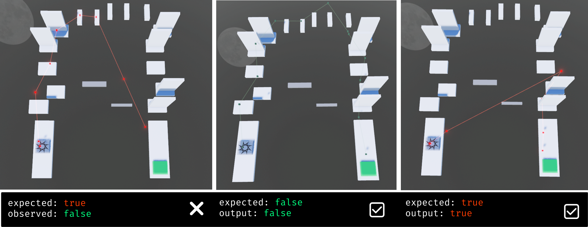
As expected with 85% accuracy, there will be some first positives like the first image. With more data, and more training, this can be easily fixed. Let’s write some final code to go ahead and save our model.

# evaluate our model on test data (in my case 85%)
model.evaluate(positions_test, is_exploiting_test)

# save it for later!
model.save("models/verycoolmodel.h5")

Closing remarks

So is this it? Is this the future of anti-cheat, should I install this into my game right now? No. The purpose of this tutorial was to learn about machine learning, and it’s potential applications on Roblox. A more practical idea may be in a drawing game with a large moderation force, you could save previous inappropriate drawings, and train a model to flag them. This way models save most of the trouble, but there’s still a human in the loop to catch errors.

Machine learning has become quite a mysterious and rapidly developing practice, and with all the misinformation and fear-mongering, I think it’s important for people to learn the inner mechanisms, realize it’s just math, and appreciate its potential helpfulness.

The Code

Place File: https://github.com/acuaroo/LTAATCE/blob/master/placefile.rbxl
Github Repo: https://github.com/acuaroo/LTAATCE

Let's teach an AI to catch exploiters!